Triple Integrals
Contents
Triple Integrals#
Triple integral on a box#
Consider a function \(f(x, y, z)\) continuous on a box \(B=[a, b] \times[c, d] \times[r, s]\).
We can define a triple Riemann sum and triple integral:
The triple integral can be evaluated by using iterated integrals and ‘partial integration’: integrating with respect to one variable while holding the other two variables constant.
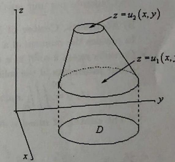
Triple integrals on general regions#
Suppose region \(E\) lies between surfaces \(z=u_{1}(x, y)\) and \(z=u_{1}(x, y)\), and that \(D\) is the projection of \(E\) onto the \(x y\)-plane, so
then
If \(D\) is a type I region, \(D=\left\{(x, y): a \leq x \leq b, g_{1}(x) \leq y \leq g_{2}(x)\right\}\), then
(Alternatively D may be type II or may be best described using plane polar coordinates.)
Iterated integrals can be written in a similar way for other situations.
Constructing and evaluating triple integrals#
Determining the limits of integration is usually the most difficult step!
When possible, it is helpful to sketch two diagrams:
A diagram of the 3D region.
Sketch of the 2D projection of the region onto the xy-plane (or other plane, as appropriate).
There is often more than one way of writing the integral … but one form may be easier to evaluate than others.
Note: The limits on the outermost integral must be constants. The limits on inner integrals can be only in terms of the remaining variables.
Further applications of multiple integrals#
Density and Mass#
Suppose a solid occupies a region \(E\) and the density (mass per unit volume) varies with position according to the function: \(\rho(x, y, z)\). A differential volume element \(d V\) at \((x, y, z)\) will have mass \(d m=\rho(x, y, z) d V\). The total mass of the solid is therefore \(m=\iiint_{E} \rho(x, y, z) d V\).
Similarly for a thin, flat plate in a region \(D\) of the \(x y\)-plane we can consider (areal) density (mass per unit area): \(\rho_{s}(x, y)\). A differential area element \(d A\) at \((x, y)\) will have mass \(d m=\rho_{s}(x, y) d A\). The mass of the plate will therefore be \(m=\iint_{D} \rho_{s}(x, y) d A\).
The ideas above can be extended to other types of densities. For example, if electric charge is distributed in a 3D region \(E\) we may consider the charge density \(\sigma(x, y, z\) ) (in Coulombs per unit volume). The total charge in region \(E\) will be \(Q=\iiint_{E} \sigma(x, y, z) d V\). Or if electric charge is distributed over a 2D surface \(D\) with surface charge density \(\sigma_{s}(x, y)\) (in Coulombs per unit area), the total charge will be \(Q=\iint_{D} \sigma_{s}(x, y) d A\).
Moments, Center of Mass and Centroid#
In physics the moment of a particle with mass \(m\) about an axis at a distance \(r\) is \(m r\).
Consider again a solid in a region \(E\) with density \(\rho(x, y, z)\).
The moments of the solid about the three coordinate planes are
The center of mass is at \((\bar{x}, \bar{y}, \bar{z})\) where
and \(m\) is the total mass of the solid (found by the integral given in i) above).
For a solid of uniform density, the center of mass is called the centroid. That is, the centroid of the solid is at \((\bar{x}, \bar{y}, \bar{z})\) where \(\bar{x}=\frac{M_{Y Z}}{m}=\frac{1}{m} \iiint_{E} x d V\), etc.
Probability#
(Review) The probability that a single continuous random variable \(X\) takes values between \(a\) and \(b\) is found by evaluating an integral \(P(a \leq X \leq b)=\int_{a}^{b} p(x) d x\) where \(p\) is a probability density function and has the properties \(\quad p(x) \geq 0 \quad \forall x \quad\) and \(\int_{-\infty}^{\infty} p(x) d x=1\).
In this case the mean or expected value, of \(X\) is \(\mu=\int_{a}^{b} x p(x) d x\).
Similarly, if we have two continuous random variables \(X\) and \(Y\) then the probability that \((X, Y)\) take values lying in a particular region \(R\) is found by evaluating an integral \(P((X, Y) \in R)=\iint_{R} p(x, y) d A \quad\) where \(p(x, y)\) is a joint probability density function and has the properties \(p(x, y) \geq 0\) and \(\int_{-\infty}^{\infty} \int_{-\infty}^{\infty} p(x, y) d x d y=1\)
The expected values of \(X\) are \(Y\) are