Line & Surface Integrals
Contents
Line & Surface Integrals#
Arc Length (revisited)#
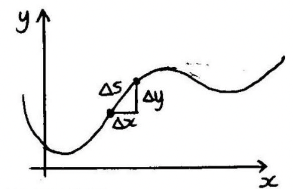
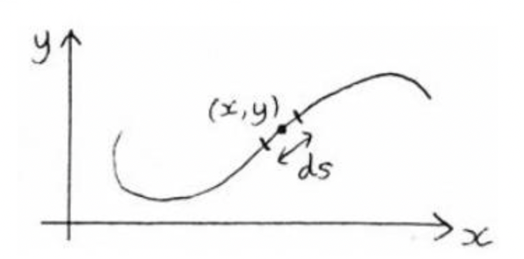
In single-variable calculus we learned that for a smooth curve \(C\) in the \(x y\)-plane, the arc length is given by an integral \(L=\int_{C} d s\) where \(d s\), the differential element of arc length, is given by \(d s=\) \(\sqrt{(d x)^{2}+(d y)^{2}}\).
For a curve \(y=f(x)\), we can write \(d s=\sqrt{(d x)^{2}+(d y)^{2}}=\sqrt{1+\left(\frac{d y}{d x}\right)^{2}} d x\), so the arc length of \(y=f(x)\) on \(a \leq x \leq b\) is given by \(L=\int_{a}^{b} \sqrt{1+\left(\frac{d y}{d x}\right)^{2}} d x\).
Similarly, for a curve \(x=g(y)\) on \(c \leq y \leq d\) we can write \(d s=\sqrt{\left(\frac{d x}{d y}\right)^{2}+1} d y\), so the arc length is \(L=\int_{c}^{d} \sqrt{\left(\frac{d x}{d y}\right)^{2}+1} d y\).
For a 2D parametric curve \(x=f(t), y=g(t), a \leq t \leq b\) we can write \(d s=\sqrt{\left(\frac{d x}{d t}\right)^{2}+\left(\frac{d y}{d t}\right)^{2}} d t\), so the arc length is \(L=\int_{a}^{b} \sqrt{\left(\frac{d x}{d t}\right)^{2}+\left(\frac{d y}{d t}\right)^{2}} d t=\int_{a}^{b} \sqrt{\left(f^{\prime}(t)\right)^{2}+\left(g^{\prime}(t)\right)^{2}} d t \quad\) [1].
Similarly for a smooth 3D curve with vector equation \(\overrightarrow{\boldsymbol{r}}(t)=\langle f(t), g(t), h(t)\rangle, a \leq t \leq b\), \(L=\int_{a}^{b} \sqrt{\left(\frac{d x}{d t}\right)^{2}+\left(\frac{d y}{d t}\right)^{2}+\left(\frac{d z}{d t}\right)^{2}} d t=\int_{a}^{b} \sqrt{\left(f^{\prime}(t)\right)^{2}+\left(g^{\prime}(t)\right)^{2}+\left(h^{\prime}(t)\right)^{2}} d t \quad[2] .\)
Results [1] and [2] are often written more concisely as \(L=\int_{a}^{b}\left|\overrightarrow{\boldsymbol{r}}^{\prime}(t)\right| d t \quad[3]\).
Optional Further Reading: Arc length parameterization and curvature
We have seen that a given curve many be parameterized many different ways, and that the parameterization affects the speed at which the curve is traversed. Arc length parameterization is a special type of parameterization such that the curve is traversed at unit speed (that is, for every unit increase in the parameter we travel one unit of distance along the curve). Such parameterisations can also be used to calculate the curvature of a curve at a point: the rate at which the curve (and its tangent vector) changes direction at that point. For more details see Thomas 13.4.
Line Integrals of Scalar Fields (with respect to arc length)#
If \(f(x, y, z)\) is defined on a smooth curve \(C \subset R^{3}\) then the line integral of \(f\) along \(C\) is \(\int_{C} f(x, y, z) d s\)
Line integrals of scalar fields are evaluated in a similar way to arc length integrals. e.g. For a 3D curve \(\overrightarrow{\boldsymbol{r}}(t)=\langle f(t), g(t), h(t)\rangle, a \leq t \leq b\), we have
Hence to evaluate a line integral, the first step is often to parameterize the curve.
If \(C\) is a piecewise smooth curve, i.e. it is composed of a finite number of smooth curves \(C_{1}, C_{2}, \ldots, C_{n}\) linked end to end, then \(\int_{C} f d s=\int_{C_{1}} f d s+\int_{C_{2}} f d s+\ldots+\int_{C_{n}} f d s\).
An application
\(\quad\) Suppose we have a thin wire shaped like a curve \(C\) in the \(x y\)-plane and that its density at \((x, y)\) is \(\rho(x, y)\).
Length element \(d s\) at \((x, y)\) has mass \(d m=\rho(x, y) d s\).
So the mass of the whole wire is \(m=\int_{C} d m=\int_{C} \rho(x, y) d s\)
The center of mass of the wire is located at \((\bar{x}, \bar{y})\), where
These three integrals are examples of line integrals of scalar fields.